Latest Page Update: 23-09-2026

Image rotation¶

One of the most useful and simple geometric transformation is rotation, where an image is rotated around a point.

We start by some experiments on the image called NusaPenida.png. It can be found in the exercise material.

Exercise 1¶

Read the NusaPenida.png image and call it im_org. It can be rotated by:

# angle in degrees - counter clockwise
rotation_angle = 10
rotated_img = rotate(im_org, rotation_angle)
show_comparison(im_org, rotated_img, "Rotated image")

Notice, that in this function, the angle should be given in degrees.

By default, the image is rotated around the center of the image. This can be changed by manually specifying the point that the image should be rotated around (here (0, 0)):

rot_center = [0, 0]
rotated_img = rotate(im_org, rotation_angle, center=rot_center)

Exercise 2¶

Experiment with different center points and notice the results.

As seen, there are areas of the rotated image that is filled with a background value. It can be controlled how this background filling shall behave.

Here the background filling mode is set to reflect

rotated_img = rotate(im_org, rotation_angle, mode="reflect")

Exercise 3¶

Try the rotation with background filling mode reflect and wrap and notice the results and differences.

Info

It is also possible to define a constant fill value. Currently, sci-kit image only supports a single value (not RGB).

Exercise 4¶

Try to use:

rotated_img = rotate(im_org, rotation_angle, resize=True, mode="constant", cval=1)

with different values of cval and notice the outcomes.

By default, the rotated output image has the same size as the input image and therefore some parts of the rotated image are cropped away. It is possible to automatically adjust the output size, so the rotated image fits into the resized image.

Exercise 5¶

Test the use of automatic resizing:

rotated_img = rotate(im_org, rotation_angle, resize=True)

also combine resizing with different background filling modes.

Euclidean image transformation¶

An alternative way of doing geometric image transformations is to first construct the transformation and then apply it to the image. We will start by the Euclidean image transformation that consists of a rotation and a translation. It is also called a rigid body transformation.

Exercise 6¶

Start by defining the transformation:

# angle in radians - counter clockwise
rotation_angle = 10.0 * math.pi / 180.
trans = [10, 20]
tform = EuclideanTransform(rotation=rotation_angle, translation=trans)
print(tform.params)

it can be seen in the print statement that the transformation consists of a 3 x 3 matrix. The matrix is used to transform points using homogenous coordinates. Notice that the angle is defined in radians in this function.

Exercise 7¶

The computed transform can be applied to an image using the warp function:

transformed_img = warp(im_org, tform)

Try it.

Info

The warp function actually does an inverse transformation of the image, since it uses the transform to find the pixels values in the input image that should be placed in the output image.

Inverse transformation¶

It is possible to get the inverse of a computed transform by using tform.inverse. An image can then be transformed using the inverse transform by:

transformed_img = warp(im_org, tform.inverse)

Exercise 8¶

Construct a Euclidean transformation with only rotation. Test the transformation and the invers transformation and notice the effect.

Similarity transform of image¶

The SimilarityTransform computes a transformation consisting of a translation, rotation and a scaling.

Exercise 9¶

Define a SimilarityTransform with an angle of \(15^o\), a translation of (40, 30) and a scaling of 0.6 and test it on the image.

The swirl image transformation¶

The swirl image transform is a non-linear transform that can create interesting visual results on images.

Exercise 10¶

Try the swirl transformation:

str = 10
rad = 300
swirl_img = swirl(im_org, strength=str, radius=rad)

it is also possible to change the center of the swirl:

str = 10
rad = 300
c = [500, 400]
swirl_img = swirl(im_org, strength=str, radius=rad, center=c)

try with different centers and notice the results.

Landmark based registration¶

The goal of landmark based registration is to align two images using a set of landmarks placed in both images. The landmarks need to have correspondence meaning that the landmarks should be placed on the same anatomical spot in the two images.

There are two photos of hands: Hand1.jpg and Hand2.jpg and the goal is to transform Hand1 so it fits on top of Hand2. In this exercise we call Hand1 one for the source (src) and Hand2 for the destination (dst).

Exercise 11¶

Start by reading the two images into src_img and dst_img. Visualize their overlap by:

blend = 0.5 * img_as_float(src_img) + 0.5 * img_as_float(dst_img)
io.imshow(blend)
io.show()

Manual landmark annotation¶

We will manually placed landmarks on the two images to align the them.

Exercise 12¶

We have manually placed a set of landmarks on the source image. They can be visualized by:

src = np.array([[588, 274], [328, 179], [134, 398], [260, 525], [613, 448]])

plt.imshow(src_img)
plt.plot(src[:, 0], src[:, 1], '.r', markersize=12)
plt.show()

Exercise 13¶

You should now place the same landmarks on the destination image.

In imshow you can see the pixel coordinates of the cursor:

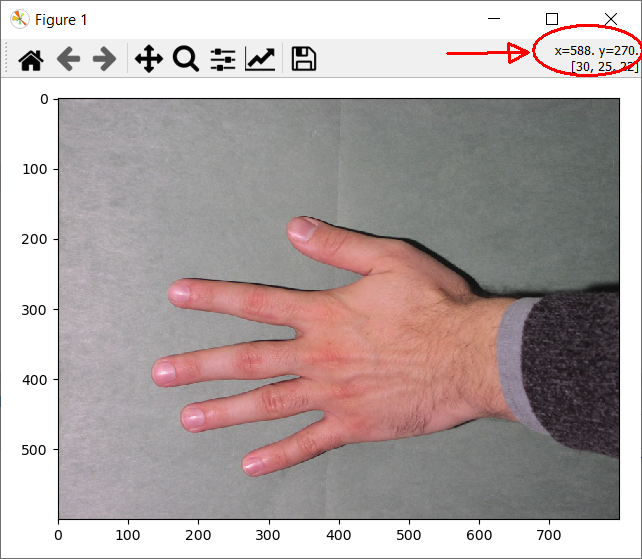
Use this to find the coordinates of the sought landmarks and put them into a dst variable.

Plot the landmarks to verify they are correct:

fig, ax = plt.subplots()
ax.plot(src[:, 0], src[:, 1], '-r', markersize=12, label="Source")
ax.plot(dst[:, 0], dst[:, 1], '-g', markersize=12, label="Destination")
ax.invert_yaxis()
ax.legend()
ax.set_title("Landmarks before alignment")
plt.show()

To calculate how well two sets of landmarks are aligned, we can compute the objective function:

\[ F = \sum_{i=1}^N \|a_i - b_i\|^2 \enspace ,\]

here \(a_i\) are the landmarks in the destination image and \(b_i\) are the landmarks in the source image.

Exercise 14¶

Compute \(F\) from your landmarks. It can for example be done like:

e_x = src[:, 0] - dst[:, 0]
error_x = np.dot(e_x, e_x)
e_y = src[:, 1] - dst[:, 1]
error_y = np.dot(e_y, e_y)
f = error_x + error_y
print(f"Landmark alignment error F: {f}")

The optimal Euclidean transformation that brings the source landmarks over in the destination landmarks can be found by:

tform = EuclideanTransform()
tform.estimate(src, dst)

The found transform can be applied to the source points by:

src_transform = matrix_transform(src, tform.params)

Exercise 15¶

Visualize the transformed source landmarks together with the destination landmarks. Also compute the objective function \(F\) using the transformed points. What do you observe?

Exercise 16¶

We can now apply the transformation to the source image. Notice that we use the inverse transform due to the inverse mapping in the image resampling:

warped = warp(src_img, tform.inverse)

Show the warped image and also try to blend the warped image destination image like in exercise 11. What do you observe?

Video transformations¶

Now try to make a small program, that acquires video from your webcam/telephone, transforms it and shows the output. In Imports and Functions there is a program that can be modified.

By default, the program acquires a colour image and rotates it. There is a counter that is increased every frame and that counter can be used to modify the transformation (for example the rotation angle). The program also measures how many milliseconds the image processing takes.

Exercise 17¶

Run the example program and notice how the output image rotates.

Exercise 18¶

Modify the program so it performs the swirl transform on the image. The parameters of the swirl transform can be changed using the counter. For example:

str = math.sin(counter / 10) * 10

Try this and also try to change the other transform parameters using the counter.

Exam preparation¶

Below are some example exam exercises related to this weeks material. Work with them, and if you have issues or questions, please ask the TAs, as you will not be able to get help after the last exercise round.

To be able to do a landmark-based image registration between a reference image and a template image, two sets of corresponding landmarks have been placed in the two images. The landmarks can be seen in the table:

Landmarks in reference	x	y	Landmarks in template	x	y
a1	3	3	b1	6	7
a2	4	2	b2	3	7
a3	7	3	b3	2	2

Before the registration, the first point in the reference image is rotated with 11 degrees using a rotation matrix (rotating counter-clockwise).

Exam question 1: What is the squared distance objective function \(F\) between the two point-sets?

Exam question 2: The points in the reference image are translated using a translation vector of \(t=(-2, 5)\). What is the change in the squared distance objective function \(F\) between the two point-sets?

Exam question 3: A company producing farming machines wants you to develop an automated system for plant identification. The specific plant typically has red leaves and is often found on brown farmland surrounded by green crops. What could be the pipeline that you would use to solve the task?

Image acquisition, HSI color thresholding, morphological operations, BLOB analysis, feature classification
Image acquisition, landmark registration, chain coding
Binary run-length coding, PCA analysis, histogram stretching, morphological closing
Hough transformation, parametric classification, confusion matrix, grey-level run length coding
Gaussian filtering, active shape model, binary chain coding, automatic thresholding
Do not know

For the following exercise, all data is provided in data/exam_prep/. Two photos with toy figures have been taken with a standard camera (play1.png and play5.png).Five landmarks have been placed on the photos and stored in the files playfixedPoints.mat and playmovingPoints.mat.

A similarity transform (translation, rotation, and scaling) has been computed so that it aligns the moving points to the fixed points. The computed transform is applied to the play5.png photo. After the transformation, a threshold is applied to the transformed image, so pixels below 180 are assigned to foreground (1) and the pixels above 180 are background (0).

A reference image called reference.png is provided. The DICE score between the reference image and the transformed (and thresholded) image is computed.

Exam question 4: What is this DICE score?

Exam question 5: What is the Euclidean distance between the first landmark in the fixed points and the first landmark in the moving points?

Exam exercise on Hough transform¶

The five data points (x, y): (7,13), (9,10), (6,10), (6,8), (3,6)

result in the corresponding five Hough space sinograms (curves in Hough space) shown below. Two Hough space sinograms are crossing at (\(\rho\) = 0.29, \(\theta\) = \(151^\circ\)).

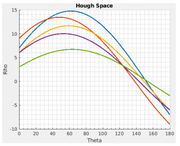
Exam question 6: What are the corresponding data points for the two crossing curves in Hough space? (approximately)

Exam exercise on dynamic programming, fall 2018¶

A gamma mapping with \(\gamma = 1.12\) is performed on the image in the below figure.

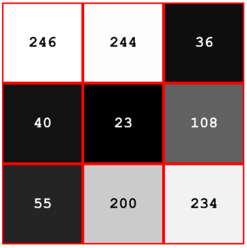
All pixels are then rounded to integers. Dynamic programming is used to compute the optimal path from the top to the bottom of the resulting image.

Exam question 7: What are the values in the lowest row in the accumulator image?