Exercises

Latest Page Update: 23-09-2026

Explorative analysis of one CT scan¶

Let us start by examining one of the CT scan slices from the training set. You can read the first slice like this:

in_dir = "data/"
ct = dicom.dcmread(in_dir + 'Training.dcm')
img = ct.pixel_array
print(img.shape)
print(img.dtype)

You should visualise the slice, so the organs of interest have a suitable brigthness and contrast. One way is to manipulate the minimum and maximum values proviede to imshow.

Exercise 1: The spleen typically has HU units in the range of 0 to 150. Try to make a good visualization of the CT scan and spleen using (replace the question marks with values):

io.imshow(img, vmin=?, vmax=?, cmap='gray')
io.show()

An expert has provided annotations of bone, fat, kidneys, liver and spleen. They are stored as mask files which is an image with the same size as the input image, where the annotated pixels are 1 and the rest are 0. They are found as BoneROI.png, FatROI.png, KidneyROI.png, LiverROI and SpleenROI.png.

You can use the original image and a mask to get the values of the pixels inside the mask:

spleen_roi = io.imread(in_dir + 'SpleenROI.png')
# convert to boolean image
spleen_mask = spleen_roi > 0
spleen_values = img[spleen_mask]

Exercise 2: Compute the average and standard deviation of the Hounsfield units found in the spleen in the training image. Do they correspond to the values found in the above figure?

Exercise 3: Plot a histogram of the pixel values of the spleen. Does it look like they are Gaussian distributed?

The function norm.pdf from SciPy represents a Gaussian probability density function (PDF). It can for example be used to plot a Gaussian distribution with a given mean and standard deviation.

This can be used to create a fitted Gaussian distribution of the spleen values:

n, bins, patches = plt.hist(spleen_values, 60, density=1)
pdf_spleen = norm.pdf(bins, mu_spleen, std_spleen)
plt.plot(bins, pdf_spleen)
plt.xlabel('Hounsfield unit')
plt.ylabel('Frequency')
plt.title('Spleen values in CT scan')
plt.show()

Here mu_spleen and std_spleen are the average and standard deviation of the spleen values.

Exercise 4: Plot histograms and their fitted Gaussians of several of the tissues types. Do they all look like they are Gaussian distributed?

The fitted Gaussians are good for inspecting class separation and how much the class overlap. Plotting several fitted Gaussians can for example be done like this:

# Hounsfield unit limits of the plot
min_hu = -200
max_hu = 1000
hu_range = np.arange(min_hu, max_hu, 1.0)
pdf_spleen = norm.pdf(hu_range, mu_spleen, std_spleen)
pdf_bone = norm.pdf(hu_range, mu_bone, std_bone)
plt.plot(hu_range, pdf_spleen, 'r--', label="spleen")
plt.plot(hu_range, pdf_bone, 'g', label="bone")
plt.title("Fitted Gaussians")
plt.legend()
plt.show()

Exercise 5: Plot the fitted Gaussians of bone, fat, kidneys, liver and spleen. What classes are easy to seperate and which classes are hard to seperate?

Exercise 6: Define the classes that we aim at classifying. Perhaps some classes should be combined into one class?

Minimum distance pixel classification¶

In the minimum distance classifier the pixel value class ranges are defined using the average values of the training values. If you have two classes, the threshold between them is defined as the mid-point between the two class value averages.

In the following, we will define four classes: background, fat, soft tissue and bone, where soft-tissue is a combination of the values of the spleen, liver and kidneys. We manually set the threshold for background to -200. So all pixels below -200 are set to background.

Exercise 7: Compute the class ranges defining fat, soft tissue and bone.

You can now use:

t_background = -200
fat_img = (img > t_background) & (img <= t_fat_soft)

to create an image where all the pixel that are classified as fat, will be 1 and the rest 0. Here t_fat_soft is the threshold between the fat and the soft tissue class.

Exercise 8: Create class images: fat_img, soft_img and bone_img representing the fat, soft tissue and bone found in the image.

To visualize the classification results you can use:

label_img = fat_img + 2 * soft_img + 3 * bone_img
image_label_overlay = label2rgb(label_img)
show_comparison(img, image_label_overlay, 'Classification result')

Exercise 9: Visualize your classification result and compare it to the anatomical image in the start of the exercise. Does your results look plausible?

Parametric pixel classification¶

In the parametric classifier, the standard deviation of the training pixel values is also used when determinin the class ranges. In the following, we are also trying to classify background, fat, soft tissue and bone.

We start by finding the class ranges by manually inspecting the fitted Gaussians from each class.

As in the last exercise, we can still se the background-fat threshold to be -200.

Exercise 10: Plot the fitted Gaussians of the training values and manually find the intersection between the curves.

Exercise 11: Use the same technique as in exercise 7, 8 and 9 to visualize your classification results. Did it change compared to the minimum distance classifier?

An alternative way of finding the class ranges is to test which class has a the highest probability for a given value. The norm.pdf function can be used for that. For example:

if norm.pdf(test_value, mu_soft, std_soft) > norm.pdf(test_value, mu_bone, std_bone):
    print(f"For value {test_value} the class is soft tissue")
else:
    print(f"For value {test_value} the class is bone")

here the test_value is a pixel value that you want to assign a class. One way to use this is to create a look-up-table where for each possible HU unit (for example 100, 101, 102 etc), the most probably class is noted. Doing this will give you the pixel value, where the two neighbouring classes meet.

Exercise 12: Use norm.pdf to find the optimal class ranges between fat, soft tissue and bone.

Object segmentation - The spleen finder¶

The goal of this part of the exercise, is to create a program that can automatically segment the spleen in CT images.

We start by using the Training.dcm image and the expert provided annotations.

Exercise 13: Inspect the values of the spleen as in exercise 3 and select a lower and upper threshold to create a spleen class range.

You can now use:

spleen_estimate = (img > t_1) & (img < t_2)
spleen_label_colour = color.label2rgb(spleen_estimate)
io.imshow(spleen_label_colour)
plt.title("First spleen estimate")
io.show()

to show your first spleen estimate. As can be seen, there a many non-spleen areas in the result. The spleen is also connected to another anatomy.

Luckily, we can use morphological operations to fix these issues.

Exercise 14: Use morphological operations to seperate the spleen from other organs and close holes. Change the values where there are question marks to change the size of the used structuring elements.

Code Template - Exercise 14

A good starting point could be:

footprint = disk(?)
closed = binary_closing(spleen_estimate, footprint)

footprint = disk(?)
opened = binary_opening(closed, footprint)

Now we can use BLOB analysis to do a feature based classification of the spleen.

Exercise 15: Use the methods from BLOB analysis to compute BLOB features for every seperated BLOB in the image.

Code Template - Exercise 15

You can for example start by:

label_img = measure.label(opened)

Exercise 16: Inspect the labeled image and validate the success of separating the spleen from the other objects. If it is connected (have the same color) to another organ, you should experiment with the kernel sizes in the morphological operations.

To be able to keep only the spleen we need to find out which BLOB features, that is special for the spleen. By using measure.regionprops many different BLOB features can be computed, including area and perimeter. You can find the catalog of available features from here.

Exercise 17: Using a combination of features and feature value limits, filter the image such that only the spleen remains in the output image.

Code Template - Exercise 17

To start, you can for example use:

min_area = ?
    max_area = ?

    # Create a copy of the label_img
    label_img_filter = label_img.copy()
    for region in region_props:
        # Find the areas that do not fit our criteria
        if region.area > max_area or region.area < min_area:
            # set the pixels in the invalid areas to background
            for cords in region.coords:
                label_img_filter[cords[0], cords[1]] = 0
    # Create binary image from the filtered label image
    i_area = label_img_filter > 0
    show_comparison(img, i_area, 'Found spleen based on area')

to create a filtered binary image, where only valid BLOBs are remaining.

Exercise 18: Create a function spleen_finder(img) that takes as input a CT image and returns a binary image, where the pixels with value 1 represent the spleen and the pixels with value 0 everything else.

Exercise 19: Test your function on the images called Validation1.dcm, Validation2.dcm and Validation3.dcm. Do you succeed in finding the spleen in all the validation images?

DICE Score¶

We would like evaluate how good we are at finding the spleen by comparing our found spleen with ground truth annotations of the spleen. The DICE score (also called the DICE coefficient or the DICE distance) is a standard method of comparing one segmentation with another segmentation.

If segmentation one is called X and the second segmentation called Y. The DICE score is computed as:

\[ \text{DICE} = \frac{2 |X \cap Y|}{|X| + |Y|} \]

where \(|X \cap Y|\) is the area (in pixels) of the overlap of the two segmentations and is \(|X| + |Y|\) the area of the union of the two segmentation. This can be visualized as:

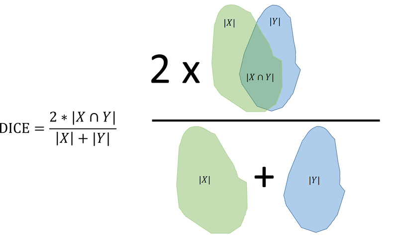
The DICE score is one if there is a perfect overlap between the two segmentations and zero if there is no overlap at all. A DICE score above 0.95 means that the two segmentations are very similar.

Using SciPy we can compute the DICE score as:

ground_truth_img = io.imread(in_dir + 'Validation1_spleen.png')
gt_bin = ground_truth_img > 0
dice_score = 1 - distance.dice(i_area.ravel(), gt_bin.ravel())
print(f"DICE score {dice_score}")

Exercise 20: Compute the DICE score for your found spleen segmentations compared to the ground truth segmentations for the three validation images. How high DICE scores do you achieve?

Testing on an independent test set¶

Overfitting occurs when an algorithm has been developed on a training set and has become so specific to that set of data, that it works badly on other similar data. To avoid this, it is necessary to test an algorithm on an independent test set. We have provided three test images Test1.dcm, Test2.dcm and Test3.dcm with ground truth spleen annotations.

Exercise 21: Use your spleen finder program to find the spleen on the three test images and compute the DICE score. What is the result of your independent test?

Exam preparation¶

Below are some example exam exercises related to this weeks material. Work with them, and if you have issues or questions, please ask the TAs, as you will not be able to get help after the last exercise round.

02502 Image Analysis Exam Fall 2022: Animal sorting machine¶

You have been asked by a farmer to develop a machine vision system that can detect if a cow or a sheep is passing by a camera. The camera just measure the average intensity of the image of the animal. To train your system, the farmer has given you these measured training data measured on 10 cows and 12 sheep:

Cows = [26, 46, 33, 23, 35, 28, 21, 30, 38, 43]

Sheep = [67, 27, 40, 60, 39, 45, 27, 67, 43, 50, 37, 100]

First, you try to compute the intensity threshold dividing cows and sheep using a minimum distance classifier. Secondly, you fit Gaussians to the two sets of the data to do a parametric classification.

Exam question 1: What threshold did you find in the minimum distance classifier?

Exam question 2: You want to find the point where the two Gaussians cross. To do that you sample values of the two Gaussians for di erent values. What are the values of the Gaussians for the cows and the sheep when trying with value=38?

02502 Image Analysis Exam Fall 2023: Heart analysis¶

A radiologist has asked you for help to assess the function of the heart as seen on a computed tomography scan. The main interest is the heart muscle (myocardium) and the blood inside the myocardium (blood). All files of interest are found in data/HeartCT.zip. We try first on a single DICOM slice (1-001.dcm), where we also have some manual annotations. We have a region-of-interest (ROI) in the myocardium (MyocardiumROI.png), a region-of-interest in the blood (bloodROI.png) and a full ground truth annotation of the blood (bloodGT.png).

Our initial analysis consist of: 1. Read the DICOM file and get the pixel values (as Hounsfield units). 2. Extract the pixel values of the ROI of the myocardium and the blood using the manual annotations.

To make an automatic segmentation of the blood, the average Hounsfield unit value (\(\mu\)) and the standard deviation (\(\sigma\)) of the Hounsfield units in the blood are computed using the manual annotations.

A class range is computed, so all pixels with:

\[\mu-3\sigma < \text{value} < \mu+3\sigma\]

Are set to foreground (1) and the rest of the pixels are set to background (0). To clean the binary image, a morphological closing with disk shaped structuring element of radius 3 is performed followed by a morphological opening with a structuring element of radius 5. A BLOB analysis is performed on the resulting image and the area of all the BLOBs are computed. The BLOBs are filtered so only BLOBs with an area larger than 2000 pixels and an area less than 5000 pixels are kept.

Finally, the found BLOB(s) are compared to the manual segmentation found in BloodGT.png and the DICE score is computed.

Exam question 3: A class range is computed, so all pixels with: \(\mu-3\sigma < \text{value} < \mu+3\sigma\) are set to foreground (1) and the rest of the pixels are set to background (0). What is the class range (in Hounsfield units)?

Exam question 4: How many BLOBs are found before they are filtered using the area?

Exam question 5: You compare your found blood estimate with the manual drawn blood estimate in BloodGT.png. What is the DICE score?