Exercises
Latest Page Update: 23-09-2026
Solution is now available! Download the full solution from here: Solution
Explorative data analysis
First we will be working with an X-ray image of the human vertebra, vertebra.png. This type of images can for example be used for diagnosis of osteoporosis. A symptom is the so-called vertebral compression fracture. However, the diagnosis is very difficult to do based on x-rays alone.
Exercise 1: Start by reading the image and inspect the histogram. Is it a bimodal histogram? Do you think it will be possible to segment it so only the bones are visible?
Solution 1
# Directory containing data and images
in_dir = "data/"
im_name = "vertebra.png"
im_org = io.imread(in_dir + im_name)
nbins = 256

fig, ax = plt.subplots(nrows=1, ncols = 2, figsize = (12, 5))
ax[0].imshow(im_org, cmap = 'gray', vmin = 0, vmax = 255)
ax[0].set_title('Image')

ax[1].hist(im_org.ravel(), bins=nbins)
ax[1].set_title('Image histogram')
ax[1].set_xlabel('Intensities')
ax[1].set_ylabel('Frequency')
plt.show()
Exercise 2: Compute the minimum and maximum values of the image. Is the full scale of the gray-scale spectrum used or can we enhance the appearance of the image?
Solution 2
fig, ax = plt.subplots(nrows=1, ncols = 2, figsize = (12, 5))
ax[0].imshow(im_org, vmin = 0, vmax = 255, cmap = 'gray')
ax[0].set_title('Visualization window: [0, 255]')
ax[1].imshow(im_org, vmin = min, vmax = max, cmap = 'gray') # Here, we change the visualization window, not the image itself!
ax[1].set_title(f'Visualization window: [{min}, {max}]')
plt.show()
Pixel type conversions
Before going further, we need to understand how to convert between between pixel types and what should be considered. A comphrehensive guide can be found here (it is not mandatory reading, we just use some highlights). One important point is that we should avoid using the astype function on images.
Conversion from unsigned byte to float image
In unsigned byte images, the possible pixel value range is [0, 255]. When converting an unsigned byte image to a float image, the possible pixel value range will be [0, 1]. When you use Python skimage function img_as_float on an unsigned byte image, it will automatically divide all pixel values with 255.
Exercise 3: Add an import statement to your script:
Read the image vertebra.png and compute and show the minumum and maximum values.
Use img_as_float to compute a new float version of your input image. Compute the minimum and maximum values of this float image. Can you verify that the float image is equal to the original image, where each pixel value is divided by 255?
Solution 3
im_float = img_as_float(im_org)
min = im_float.min()
max = im_float.max()
print(f"Min value: {min} \t Max value: {max}")

# Can you verify that the float image is equal to the original image, where each pixel value is divided by 255?
all_equal = np.allclose(im_org, im_float*255)
print(f'The float and the original image are equivalent?: {all_equal}')
Conversion from float image to unsigned byte image
As stated above, an (unsigned) float image can have pixel values in [0, 1]. When using the Python skimage function img_as_ubyte on an (unsigned) float image, it will multiply all values with 255 before converting into a byte. Remember that all decimal number will be converted into integers by this, and some information might be lost.
Exercise 4: Use img_as_ubyte on the float image you computed in the previous exercise. Compute the Compute the minimum and maximum values of this image. Are they as expected?
Solution 4
Histogram stretching
You should implement a function, that automatically stretches the histogram of an image. In other words, the function should create a new image, where the pixel values are changed so the histogram of the output image is optimal. Here optimal means, that the minimum value is 0 and the maximum value is 255. It should be based on the linear histogram stretching equation:
Here \(f(x,y)\) is the input pixel value and \(g(x,y)\) is the output pixel value, \(v_\text{max,d}\) and \(v_\text{min,d}\) are the desired minimum and maximum values (0 and 255) and \(v_\text{max}\) and \(v_\text{min}\) are the current minumum and maximum values.
Exercise 5: *Implement a Python function called histogram_stretch.
Code Template - Exercise 5
It can, for example, follow this example:*
def histogram_stretch(img_in):
    """
    Stretches the histogram of an image
    :param img_in: Input image
    :return: Image, where the histogram is stretched so the min values is 0 and the maximum value 255
    """
    # img_as_float will divide all pixel values with 255.0
    img_float = img_as_float(img_in)
    min_val = img_float.min()
    max_val = img_float.max()
    min_desired = 0.0
    max_desired = 1.0

    # Do something here

    # img_as_ubyte will multiply all pixel values with 255.0 before converting to unsigned byte
    return img_as_ubyte(img_out)
Solution 5
def histogram_stretch(img_in):
    """
    Stretches the histogram of an image
    :param img_in: Input image
    :return: Image, where the histogram is stretched so the min values is 0 and the maximum value 255
    """
    # img_as_float will divide all pixel values with 255.0
    img_float = img_as_float(img_in)
    min_val = img_float.min()
    max_val = img_float.max()
    min_desired = 0.0
    max_desired = 1.0

    # Do something here
    img_out = ((img_float-min_val)*(max_desired-min_desired)/(max_val-min_val))+min_desired
    # img_as_ubyte will multiply all pixel values with 255.0 before converting to unsigned byte
    return img_as_ubyte(img_out)
Exercise 6: Test your histogram_stretch on the vertebra.png image. Show the image before and after the histogram stretching. What changes do you notice in the image? Are the important structures more visible?
Solution 6
im_stretched = histogram_stretch(im_org)

fig, ax = plt.subplots(nrows=1, ncols = 2, figsize = (12, 5))
ax[0].imshow(im_org, cmap = 'gray', vmin = 0, vmax = 255)
ax[0].set_title('Original image')
ax[1].imshow(im_stretched, cmap = 'gray', vmin = 0, vmax = 255)
ax[1].set_title('Stretched image')
plt.show()
Non-linear pixel value mapping
The goal is to implement and test a function that performs a \(\gamma\)-mapping of pixel values:
You can use the Numpy function power to compute the actual mapping function.
Exercise 7: Implement a function, gamma_map(img, gamma), that:
- Converts the input image to float
- Do the gamma mapping on the pixel values
- Returns the resulting image as an unsigned byte image.
Solution 7
Exercise 8: Test your gamma_map function on the vertebra image or another image of your choice. Try different values of \(\gamma\), for example 0.5 and 2.0. Show the resuling image together with the input image. Can you see the differences in the images?
Solution 8
gamma_0_5 = gamma_map(im_org, 0.5)
gamma_2 = gamma_map(im_org, 2)

fig, ax = plt.subplots(nrows=1, ncols = 3, figsize = (12, 5))
ax[0].imshow(im_org, cmap = 'gray', vmin=0, vmax=255)
ax[0].set_title('Original image')
ax[1].imshow(gamma_0_5, cmap = 'gray', vmin=0, vmax=255)
ax[1].set_title(r'$\gamma = 0.5$')
ax[2].imshow(gamma_2, cmap = 'gray', vmin=0, vmax=255)
ax[2].set_title(r'$\gamma = 2$')
plt.show()
Image segmentation by thresholding
Now we will try to implement some functions that can seperate an image into segments. In this exercise, we aim at seperating the background from the foreground by setting a threshold in a gray scale image or several thresholds in color images.
Exercise 9: Implement a function, threshold_image :
def threshold_image(img_in, thres):
    """
    Apply a threshold in an image and return the resulting image
    :param img_in: Input image
    :param thres: The treshold value in the range [0, 255]
    :return: Resulting image (unsigned byte) where background is 0 and foreground is 255
    """
Remember to use img_as_ubyte when returning the resulting image.
Solution 9
def threshold_image(img_in, thres):
    """
    Apply a threshold in an image and return the resulting image
    :param img_in: Input image
    :param thres: The treshold value in the range [0, 255]
    :return: Resulting image (unsigned byte) where background is 0 and foreground is 255
    """
    mask = img_in > thres
    return img_as_ubyte(mask)
Exercise 10: Test your threshold_image function on the vertebra image with different thresholds. It is probably not possible to find a threshold that seperates the bones from the background, but can you find a threshold that seperates the human from the background?
Solution 10
im_thres = threshold_image(im_org, thres = 110)

fig, ax = plt.subplots(nrows=1, ncols = 3, figsize = (12, 5))
ax[0].imshow(im_org, cmap = 'gray', vmin = 0, vmax = 255)
ax[0].set_title('Original image')
ax[1].imshow(im_thres, cmap = 'gray', vmin = 0, vmax = 255)
ax[1].set_title('Foreground image')
ax[2].imshow(im_org, cmap = 'gray', vmin = 0, vmax = 255)
ax[2].contour(im_thres, [254, 256])
ax[2].set_title('Mask contour')
plt.show()
Automatic thresholds using Otsu's method
An optimal threshold can be estimated using Otsu's method. This method finds the threshold, that minimizes the combined variance of the foreground and background.
Exercise 11: Read the documentation of Otsu's method and use it to compute and apply a threshold to the vertebra image.
How does the threshold and the result compare to your manually found threshold?
Solution 11
from skimage.filters import threshold_otsu

thres_new = threshold_otsu(im_org)
im_thres = threshold_image(im_org, thres = thres_new)

fig, ax = plt.subplots(nrows=1, ncols = 3, figsize = (12, 5))
ax[0].imshow(im_org, cmap = 'gray', vmin = 0, vmax = 255)
ax[0].set_title('Original image')
ax[1].imshow(im_thres, cmap = 'gray', vmin = 0, vmax = 255)
ax[1].set_title(f'Foreground image [thres = {thres_new}]')
ax[2].imshow(im_org, cmap = 'gray', vmin = 0, vmax = 255)
ax[2].contour(im_thres, [254, 256])
ax[2].set_title('Mask contour')
plt.show()
Exercicse 12: Use your camera to take some pictures of yourself or a friend. Try to take a picture on a dark background. Convert the image to grayscale and try to find a threshold that creates a silhouette image (an image where the head is all white and the background black).
Tip
Alternatively, you can use the supplied photo dark_background.png found in the exercise data.
Solution 12
from skimage.color import rgb2gray

im_name = "dark_background.png"
im_org = io.imread(in_dir + im_name)

im_org = img_as_float(im_org)
im_gray = img_as_ubyte(rgb2gray(im_org))

thres = 5
im_thres = threshold_image(im_gray, thres = thres)

fig, ax = plt.subplots(nrows=1, ncols = 2, figsize = (12, 5))
ax[0].imshow(im_gray, cmap = 'gray', vmin = 0, vmax = 255)
ax[0].set_title('Original image')
ax[1].imshow(im_thres, cmap = 'gray', vmin = 0, vmax = 255)
ax[1].set_title(f'Silhouette')
plt.show()
Color thresholding in the RGB color space
In the following, we will make a simple system for road-sign detection. Start by reading the image DTUSigns2.jpg found in the exercise data. We want to make a system that do a segmentation of the image - meaning that a new binary image is created, where the foreground pixels correspond to the sign we want to detect.
We do that by tresholding the colour-channels individually. This code segments out the blue sign:
    r_comp = im_org[:, :, 0]
    g_comp = im_org[:, :, 1]
    b_comp = im_org[:, :, 2]
    segm_blue = (r_comp < 10) & (g_comp > 85) & (g_comp < 105) & \
                (b_comp > 180) & (b_comp < 200)
Exercise 13: Create a function detect_dtu_signs that takes as input a color image and returns an image, where the blue sign is identified by foreground pixels.
Solution 13
# Change the backend to be able to explore the pixel intensities
# For VSCode Notebooks and JupyterNotebook "%matplotlib widget"
# For Spyder "%matplotlib auto"

%matplotlib widget

im_name = "DTUSigns2.jpg"
im_org = io.imread(in_dir + im_name)

fig, ax = plt.subplots(nrows = 1, ncols = 1, figsize = (5,5))
ax.imshow(im_org)
plt.show()
Exercise 14: Extend your detect_dtu_signs function so it can also detect red signs. You can add an argument to the function, that tells which color it should look for.
You should use one of the explorative image tools to find out what the typical RGB values are in the red signs.
Solution 14
%matplotlib inline
plt.close()

def detect_dtu_signs(img_in, sign):
    r_comp = img_in[:, :, 0]
    g_comp = img_in[:, :, 1]
    b_comp = img_in[:, :, 2]

    if sign == 'red':
        segm = (r_comp > 160) & (r_comp < 180) & (g_comp > 50) & (g_comp < 80) & \
                    (b_comp > 50) & (b_comp < 80)
    if sign == 'blue':
        segm = (r_comp < 10) & (g_comp > 85) & (g_comp < 105) & \
                    (b_comp > 180) & (b_comp < 200)

    return img_as_ubyte(segm)


img_red = detect_dtu_signs(im_org, 'red')
fig, ax = plt.subplots(nrows = 1, ncols = 2, figsize = (10, 5))
ax[0].imshow(im_org)
ax[0].set_title('Original')
ax[1].imshow(img_red, vmin = 0, vmax = 255, cmap = 'gray')
ax[1].set_title('Red sign')
plt.show()
Color thresholding in the HSV color space
Sometimes it gives better segmentation results when the tresholding is done in HSI (also known as HSV - hue, saturation, value) space. Start by reading the DTUSigns2.jpg image, convert it to HSV and show the hue and value (from here):
    hsv_img = color.rgb2hsv(im_org)
    hue_img = hsv_img[:, :, 0]
    value_img = hsv_img[:, :, 2]
    fig, (ax0, ax1, ax2) = plt.subplots(ncols=3, figsize=(8, 2))
    ax0.imshow(im_org)
    ax0.set_title("RGB image")
    ax0.axis('off')
    ax1.imshow(hue_img, cmap='hsv')
    ax1.set_title("Hue channel")
    ax1.axis('off')
    ax2.imshow(value_img)
    ax2.set_title("Value channel")
    ax2.axis('off')

    fig.tight_layout()
    io.show()
Exercise 15: Now make a sign segmentation function using tresholding in HSV space and locate both the blue and the red sign.
Solution 15
%matplotlib widget

hsv_img = color.rgb2hsv(im_org)
hue_img = hsv_img[:, :, 0]
value_img = hsv_img[:, :, 2]
fig, (ax0, ax1, ax2) = plt.subplots(ncols=3, figsize=(8, 2))
ax0.imshow(im_org)
ax0.set_title("RGB image")
ax0.axis('off')
ax1.imshow(hue_img, cmap='hsv')
ax1.set_title("Hue channel")
ax1.axis('off')
ax2.imshow(value_img)
ax2.set_title("Value channel")
ax2.axis('off')

fig.tight_layout()
io.show()
%matplotlib inline
plt.close()

segm_blue = (hue_img < 0.6) & (hue_img  > 0.4) & (value_img < 0.77) & (value_img > 0.70)
segm_red = (hue_img < 1.0) & (hue_img  > 0.9)

fig, (ax1, ax2) = plt.subplots(1,2,figsize = (10,5))
ax1.imshow(segm_blue, cmap = 'gray')
ax1.set_title('DTU sign image (Blue)')

ax2.imshow(segm_red, cmap = 'gray')
ax2.set_title('DTU sign image (Red)')
plt.show()
Real time pixelwise operations on videos
In Imports and Functions, there is a Python script using OpenCV that:
- Connects to a camera
- Acquire images, converts them to gray-scale
- Do a simple processing on the gray-scale (inversion) or the colour image (inversion of the red channel)
- Computes the frames per second (fps) and shows it on an image.
- Shows input and resulting images in windows.
- Checks if the key
qhas been pressed and stops the program if it is pressed.
It is possible to use a mobile phone as a remote camera by following the instructions in exercise 2b.
Exercise 16: *Run the program from the exercise material and see if it shows the expected results? *
Solution 16
Run from jupyter by executing solution file:
in a code block. The solution file contains:
from skimage import color
from skimage.util import img_as_ubyte
from skimage.util import img_as_float
import time
import cv2


def show_in_moved_window(win_name, img, x, y):
    """
    Show an image in a window, where the position of the window can be given
    """
    cv2.namedWindow(win_name)
    cv2.moveWindow(win_name, x, y)
    cv2.imshow(win_name, img)


def process_gray_image(img):
    """
    Do a simple processing of an input gray scale image and return the processed image.
    # https://scikit-image.org/docs/stable/user_guide/data_types.html#image-processing-pipeline
    """
    img_float = img_as_float(img)
    img_proc = 1 - img_float
    return img_as_ubyte(img_proc)

def process_rgb_image(img):
    """
    Simple processing of a color (RGB) image
    """
    # Copy the image information so we do not change the original image
    proc_img = img.copy()
    r_comp = proc_img[:, :, 0]
    proc_img[:, :, 0] = 1 - r_comp
    return proc_img


def capture_from_camera_and_show_images():
    print("Starting image capture")

    print("Opening connection to camera")
    url = 0
    use_droid_cam = False
    if use_droid_cam:
        url = "http://192.168.1.120:4747/video"
    cap = cv2.VideoCapture(url)
    if not cap.isOpened():
        print("Cannot open camera")
        exit()

    print("Starting camera loop")
    # To keep track of frames per second using a high-performance counter
    old_time = time.perf_counter()
    fps = 0
    stop = False
    process_rgb = False
    while not stop:
        ret, new_frame = cap.read()
        if not ret:
            print("Can't receive frame. Exiting ...")
            break

        # Change from OpenCV BGR to scikit image RGB
        new_image = new_frame[:, :, ::-1]
        new_image_gray = color.rgb2gray(new_image)
        if process_rgb:
            proc_img = process_rgb_image(new_image)
            # convert back to OpenCV BGR to show it
            proc_img = proc_img[:, :, ::-1]
        else:
            proc_img = process_gray_image(new_image_gray)

        # update FPS - but do it slowly to avoid fast changing number
        new_time = time.perf_counter()
        time_dif = new_time - old_time
        old_time = new_time
        fps = fps * 0.95 + 0.05 * 1 / time_dif

        # Put the FPS on the new_frame
        str_out = f"fps: {int(fps)}"
        font = cv2.FONT_HERSHEY_COMPLEX
        cv2.putText(new_frame, str_out, (100, 100), font, 1, 255, 1)

        # Display the resulting frame
        show_in_moved_window('Input', new_frame, 0, 10)
        show_in_moved_window('Input gray', new_image_gray, 600, 10)
        show_in_moved_window('Processed image', proc_img, 1200, 10)

        if cv2.waitKey(1) == ord('q'):
            stop = True

    print("Stopping image loop")
    cap.release()
    cv2.destroyAllWindows()


if __name__ == '__main__':
    capture_from_camera_and_show_images()
Exercise 17: Change the gray-scale processing in the exercise material script to be for example thresholding, gamma mapping or something else. Do you get the visual result that you expected?
Solution 17
Run from jupyter by executing solution file:
in a code block. The solution file contains:
from skimage import color
from skimage.filters import threshold_otsu
from skimage.util import img_as_ubyte
from skimage.util import img_as_float
import numpy as np
import time
import cv2


def show_in_moved_window(win_name, img, x, y):
    """
    Show an image in a window, where the position of the window can be given
    """
    cv2.namedWindow(win_name)
    cv2.moveWindow(win_name, x, y)
    cv2.imshow(win_name, img)


def process_gray_image(img):
    """
    Apply some basic processing to get a the foreground from the image
    """
    img_float = img_as_float(img)
    img_gamma = np.power(img_float, 2)

    thres_new = threshold_otsu(img_gamma)
    mask = img_gamma > thres_new
    return img_as_ubyte(mask)

def process_rgb_image(img):
    """
    Simple processing of a color (RGB) image
    """
    # Copy the image information so we do not change the original image
    proc_img = img.copy()
    r_comp = proc_img[:, :, 0]
    proc_img[:, :, 0] = 1 - r_comp
    return proc_img


def capture_from_camera_and_show_images():
    print("Starting image capture")

    print("Opening connection to camera")
    url = 0
    use_droid_cam = False
    if use_droid_cam:
        url = "http://192.168.1.120:4747/video"
    cap = cv2.VideoCapture(url)
    if not cap.isOpened():
        print("Cannot open camera")
        exit()

    print("Starting camera loop")
    # To keep track of frames per second using a high-performance counter
    old_time = time.perf_counter()
    fps = 0
    stop = False
    process_rgb = False
    while not stop:
        ret, new_frame = cap.read()
        if not ret:
            print("Can't receive frame. Exiting ...")
            break

        # Change from OpenCV BGR to scikit image RGB
        new_image = new_frame[:, :, ::-1]
        new_image_gray = color.rgb2gray(new_image)
        if process_rgb:
            proc_img = process_rgb_image(new_image)
            # convert back to OpenCV BGR to show it
            proc_img = proc_img[:, :, ::-1]
        else:
            proc_img = process_gray_image(new_image_gray)

        # update FPS - but do it slowly to avoid fast changing number
        new_time = time.perf_counter()
        time_dif = new_time - old_time
        old_time = new_time
        fps = fps * 0.95 + 0.05 * 1 / time_dif

        # Put the FPS on the new_frame
        str_out = f"fps: {int(fps)}"
        font = cv2.FONT_HERSHEY_COMPLEX
        cv2.putText(new_frame, str_out, (100, 100), font, 1, 255, 1)

        # Display the resulting frame
        show_in_moved_window('Input', new_frame, 0, 10)
        show_in_moved_window('Input gray', new_image_gray, 600, 10)
        show_in_moved_window('Processed image', proc_img, 1200, 10)

        if cv2.waitKey(1) == ord('q'):
            stop = True

    print("Stopping image loop")
    cap.release()
    cv2.destroyAllWindows()


if __name__ == '__main__':
    capture_from_camera_and_show_images()
Exercise 18: Real time detection of DTU signs
Change the rgb-scale processing in the exercise material script so it does a color threshold in either RGB or HSV space. The goal is to make a program that can see DTU street signs. The output should be a binary image, where the pixels of the sign is foreground. Later in the course, we will learn how to remove the noise pixels.
Solution 18
Run from jupyter by executing solution file:
in a code block. The solution file contains:
from skimage import color
from skimage.filters import threshold_otsu
from skimage.util import img_as_ubyte
from skimage.util import img_as_float
import numpy as np
import time
import cv2


def show_in_moved_window(win_name, img, x, y):
    """
    Show an image in a window, where the position of the window can be given
    """
    cv2.namedWindow(win_name)
    cv2.moveWindow(win_name, x, y)
    cv2.imshow(win_name, img)


def process_hsv_image(img):
    """
    Simple processing of a color (HSV) image
    """
    hue_img = img[:, :, 0]
    segm_red = (hue_img < 1.0) & (hue_img  > 0.9)
    return img_as_ubyte(segm_red)

def process_rgb_image(img):
    """
    Segmentation of red structures in the RGB channel
    """
    r_comp = img[:, :, 0]
    g_comp = img[:, :, 1]
    b_comp = img[:, :, 2]

    segm = (r_comp > 160) & (r_comp < 180) & (g_comp > 50) & (g_comp < 80) & \
                (b_comp > 50) & (b_comp < 80)

    return img_as_ubyte(segm)


def capture_from_camera_and_show_images():
    print("Starting image capture")

    print("Opening connection to camera")
    url = 0
    use_droid_cam = False
    if use_droid_cam:
        url = "http://192.168.1.120:4747/video"
    cap = cv2.VideoCapture(url)
    if not cap.isOpened():
        print("Cannot open camera")
        exit()

    print("Starting camera loop")
    # To keep track of frames per second using a high-performance counter
    old_time = time.perf_counter()
    fps = 0
    stop = False
    process_rgb = False
    while not stop:
        ret, new_frame = cap.read()
        if not ret:
            print("Can't receive frame. Exiting ...")
            break

        # Change from OpenCV BGR to scikit image RGB
        new_image = new_frame[:, :, ::-1]
        if process_rgb:
            mask_red = process_rgb_image(new_image)
        else:
            new_image = color.rgb2hsv(new_image)
            mask_red = process_hsv_image(new_image)

        # update FPS - but do it slowly to avoid fast changing number
        new_time = time.perf_counter()
        time_dif = new_time - old_time
        old_time = new_time
        fps = fps * 0.95 + 0.05 * 1 / time_dif

        # Put the FPS on the new_frame
        str_out = f"fps: {int(fps)}"
        font = cv2.FONT_HERSHEY_COMPLEX
        cv2.putText(new_frame, str_out, (100, 100), font, 1, 255, 1)

        # Display the resulting frame
        show_in_moved_window('Input', new_frame, 0, 10)
        show_in_moved_window('Mask', mask_red, 600, 10)
        if cv2.waitKey(1) == ord('q'):
            stop = True

    print("Stopping image loop")
    cap.release()
    cv2.destroyAllWindows()


if __name__ == '__main__':
    capture_from_camera_and_show_images()
Exam preparation
Below are some example exam exercises related to this weeks material. Work with them, and if you have issues or questions, please ask the TAs, as you will not be able to get help after the last exercise round.
Exercise from 02502 Image Analysis Spring 2021 exam
Exam question 1: The photo called sky_gray.png (in data/) is loaded and a linear histogram stretching is performed so the new image has a maximum pixel value of 200 and a minimum pixel value of 10. What is the average pixel value of the new image?
- 87
- 98
- 113
- 167
- 103
Solution 19
- 87
- 98
- 113
- 167
- 103
Exercise from 02502 Image Analysis Fall 2022 exam
You are testing a prototype of a system that can monitor car parking areas. In order to locate the cars you want to create a binary image. Your algorithm does:
- Converts the input image from RGB to gray scale and transforms it into a floating point image.
- Does a linear gray scale transformation so the transformed image has a minimum pixel value of 0.1 and a maximum pixel value of 0.6
- Computes a pixel value threshold using Otsu's method
- Applies the found threshold, so all pixels with values above the threshold becomes foreground (white) and the rest background (black).
You test your algorithm on the supplied photo (data/pixelwise.png)
Exam question 2: What is the threshold value found by Otsu method?
- 0.17
- 0.37
- 0.33
- Do not know
- 0.21
- 0.49
Solution 20
- 0.17
- 0.37
- 0.33
- Do not know
- 0.21
- 0.49
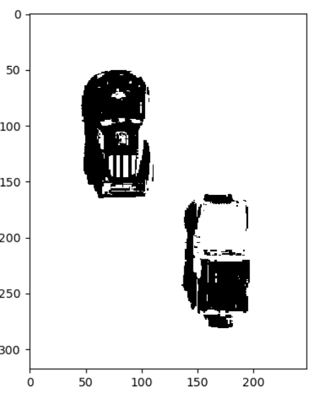
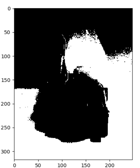
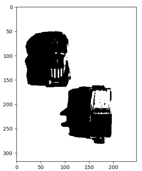
Exam question 3: What is the resulting binary image, when applying your algorithm to the test photo?
- Figure 1:
- Figure 2:
- Figure 3:
Solution 21
- Figure 1
- Figure 2
- Figure 3
Exam question 4: You are working with quality assurance of printing of industrial products. As a test you want to see the color quality of printing on tea bags (data/TeaBag.png). You have developed a simple method that produces the image below. What are the steps in your pipeline?
- Load image, RGB to grayscale, Otsu's optimal threshold
- Do not know
- Load image, RGB to HSV, threshold with 230 on V component
- Load image, RGB thresholding with R < 100, G < 100, and B > 100
Solution 22
- Load image, RGB to grayscale, Otsu's optimal threshold
- Do not know
- Load image, RGB to HSV, threshold with 230 on V component
- Load image, RGB thresholding with R < 100, G < 100, and B > 100